Takashi Unuma's blog.

Home About Archive

Polarimetric Radar Observation Operator

はじめに

前回、Spectral Bin Microphysics Model にて、気象数値モデルを用いた粒形分布の計算例を示した。以前、粒径分布とレーダー変数で示したように、レーダー変数もまた粒形分布から計算可能である。そこで、今回は Spectral Bin Microphysics Model で出力したデータを用い、レーダー変数を計算・描画することを試みる。

Cloud Resolving Model Radar Simulator

雲解像モデルを用いたレーダー変数の計算は、いくつかの方法が提案されている。最近では、パッケージ化されたものが開発されてきている。中でも Cloud Resolving Model Radar Simulator (CR-SIM; Oue et al. 2020) は、GNU PUBLIC LICENSE で利用可能なツールの一つである。2020年6月20日時点の最新版は 3.33 となっている。Stony Brook University の Web ページからダウンロードが可能。ただし、ファイルサイズが約 13 GB と少々大きいので、ダウンロード時の回線速度やパケット容量に注意が必要。今回は、レーダー変数の計算に必要なコアパッケージ crsim-3.33.tar.gz のみをダウンロードした。

プログラムの修正

tar.gz ファイルを展開後、そのままコンパイルするだけではエラーを吐くので、下記を修正する。

diff --git a/share/crsim/test/Makefile.in b/share/crsim/test/Makefile.in
index 3b862a3..1fb76f5 100644
--- a/share/crsim/test/Makefile.in
+++ b/share/crsim/test/Makefile.in
@@ -195,21 +195,19 @@ target_alias = @target_alias@
 top_build_prefix = @top_build_prefix@
 top_builddir = @top_builddir@
 top_srcdir = @top_srcdir@
-TESTS = run_test1.sh run_test2.sh run_test3.sh run_test4.sh
+TESTS = run_test1.sh run_test2.sh run_test3.sh
 EXTRA_DIST = run_test1.sh.in \
              run_test2.sh.in \
-             run_test3.sh.in \
-             run_test4.sh.in
+             run_test3.sh.in

 auxdir = $(datadir)/crsim/test
 ddir = .$(pwd)
 edit = sed -e 's|@nccmp[@]|$(NCCMP)|g'
 nobase_dist_aux_DATA = run_test1.sh \
                         run_test2.sh \
-                        run_test3.sh \
-                        run_test4.sh
+                        run_test3.sh

-CLEANFILES = run_test1.sh run_test2.sh run_test3.sh run_test4.sh
+CLEANFILES = run_test1.sh run_test2.sh run_test3.sh
 all: all-am

 .SUFFIXES:
@@ -522,21 +520,16 @@ run_test2.sh: run_test2.sh.in Makefile
 run_test3.sh: run_test3.sh.in Makefile
        $(edit) '$(srcdir)/$@.in' > $@
        chmod 755 run_test3.sh
-run_test4.sh: run_test4.sh.in Makefile
-       $(edit) '$(srcdir)/$@.in' > $@
-       chmod 755 run_test4.sh

 install-data-hook:
        chmod a+rx $(auxdir)/run_test1.sh
        chmod a+rx $(auxdir)/run_test2.sh
        chmod a+rx $(auxdir)/run_test3.sh
-       chmod a+rx $(auxdir)/run_test4.sh

 installcheck-local:
        cd $(auxdir) && sh run_test1.sh
        cd $(auxdir) && sh run_test2.sh
        cd $(auxdir) && sh run_test3.sh
-       cd $(auxdir) && sh run_test4.sh

 # Tell versions [3.59,3.63) of GNU make to not export all variables.
 # Otherwise a system limit (for SysV at least) may be exceeded.
diff --git a/src/crsim_subrs.f90 b/src/crsim_subrs.f90
index 4539fe4..9c9120b 100644
--- a/src/crsim_subrs.f90
+++ b/src/crsim_subrs.f90
@@ -4023,6 +4023,7 @@
       if (conf%MP_PHYSICS==9)  den_string='800' !changed by oue because mpl lut does not includes 840 2017/12/08
       if (conf%MP_PHYSICS==10) den_string='500'
       if (conf%MP_PHYSICS==8)  den_string='900' !Added by oue 2016/09/16: Note that Thopmson scheme assumes ice density of 890
+      if (conf%MP_PHYSICS==20)  den_string='400' !Added for HUCM SBM
       if (conf%MP_PHYSICS==30)  den_string='400' !Added by oue 2017/07/17:
       if (conf%MP_PHYSICS==40)  den_string='400' !Added by oue 2017/07/21:
       if (conf%MP_PHYSICS==50)  den_string='900' !Added by DW for P3

Makefile.in の run_test4.sh はテスト用のサンプルデータが同梱されておらず実行不可だったので、除外した。また、WRF-SBM の結果を用いる場合、条件分岐に抜けがあったので暫定値を追加した。

動作環境

Rocky Linux 8.9 x86_64
GNU compiler version 8.5.0
NetCDF-C version 4.7.0
NetCDF-Fortran version 4.5.2
HDF5 version 1.10.5
ZLIB version 1.2.11

コンパイル

make check 時に NCCMP が必要となるので、事前にインストールしておく。また、tar.gz ファイルを展開すると、数十 GB 程度に肥大するので、ディスク容量に十分な空きスペースがあることも確認しておく。また、configure の前に FCFLAGS と CFLAGS の環境変数を設定しておく。

export FCFLAGS=$(nc-config --fflags) && export CFLAGS=$(nc-config --cflags)

設定出来たら、NetCDF, NetCDF-Fortran, NCCMP, インストール先のそれぞれのディレクトリを指定した上で configure を実行。

./configure --with-netcdf=/usr --with-netcdf-fortran=/usr --with-nccmp=/work/nccmp/bin --prefix=/work/crsim-3.33

Makefile が作成されたら、make でコンパイル。

make

続いて、test case を実行し、結果が nccmp でバイナリ一致することを確認。

make check

問題なければ、make install を実行する。

make install

指定したディレクトリ以下に bin/ etc/ share/ がそれぞれあれば OK。

パラメーターファイル

PARAMETERS に設定を書き込む仕様となっている。サンプルファイルは、インストール先の etc 以下にある。以下、今回利用するパラメーター例。

# PARAMETERS CR-SIM v3.2x
# speccify the number of OpenMP threads used in the code (integer, OMPThreadNum)
1
# specify the starting and ending indices of domain and desired saved time step: ix_start,ix_end, iy_start,iy_end, iz_start,iz_end,it. If negative, all points in specific direction are used( 1-> nx, 1-> ny, 1->nz, respectivelly.
1,41
1,41
1,40    # iz_start,iz_end
1       # it
# specify the microphysics Morrison 10, JFan 20, Milbranndt-Yau 9 with snow spherical,optionally 901 for Milbranndt-Yau with snow not spherical, P3 50, and Thompson 8 (modified by DW)
20
# specify the indices of radar position ixc,iyc. if ixc=-999, radar locations are every grid box at iyc, iyc=-999, radar locations are every grid box at ixc.
20,20
# specify the height of radar in meters
1000.d0
#Specify the file of ice PSD parameters for P3 microphysics scheme (added by DW)
#"./../aux/p3_ice_psd_para_lookup_table.dat" #(added by DW)
#assign the scattering type to each hydrometeor (5 lines for MP_PHYSICS=10,20; 6 lines for MP_PHYSICS=9 and 50). Order has to be 1-cloud, 2-rain, 3-ice, 4-snow, 5-graupel and 6 -hail. (For P3, order has to be 1-cloud, 2-rain, 3-small ice, 4-unrimed ice, 5-graupel and 6-partial rimed ice.) (modified by DW)
"cloud"
"rainb"
"ice_ar0.20"
"snow_ar0.60"
"gh_ryzh"
#assign the minimum thresholds of the input mixing ratio for the radar simulation. The input values of mixing ratios <= specified threshold will be set to 0. Order has to be 1-cloud, 2-rain, 3-ice, 4-snow, 5-graupel and 6 -hail. (For P3, order has to be 1-cloud, 2-rain, 3-small ice, 4-unrimed ice, 5-graupel and 6-partial rimed ice.) (modified by DW)
1.d-8
1.d-8
1.d-11
1.d-11
1.d-8
# horienID (integer),sigma(double precis.) for each hydrometeor category  - choice of orientation distribution (1=chaotic,2=random orientation in the horizontal plane, 3=2D Gaussian with zero mean and sigma standard deviation). In the case those values are negative, the default value are used. If horienID /=3, sigma values are disregarded.Order has to be 1-cloud, 2-rain, 3-ice, 4-snow, 5-graupel (and 6 -hail). (For P3, order has to be 1-cloud, 2-rain, 3-small ice, 4-unrimed ice, 5-graupel and 6-partial rimed ice.) (modified by DW)
3,10.d0
3,10.d0
3,10.d0
3,40.d0
3,40.d0
# Specify radar frequency (3.0d0, 5.5d0, 9.5d0, 35.0d0, 94.0d0)
5.5d0
# Specify elevation, if this ranges from -90 to 90, elevation has a fixed value; if -999, elevation of each pixel is relative to radar origin given by indices (ixc,iyc)
0.7d0
##turn off the polaraimetric variables : yes ==1 , any other number no
0
# Specify radar beamwidth ( i.e one-way angular resolution Theta1) in degrees
0.1d0
# Specify the radar range resolution dr in meters (= (c Tau) / 2 )
250.d0
# Specify value of coefficient ZMIN in relation dBZ_min(dBZ)=ZMIN(dBZ)+20 log10(range in km)
-50.d0
# Introduce cloud lidar (ceilometer,fr=905 nm) ceiloID=0 no; =1 yes
0
# Introduce micropulse lidar (MPL) mplID =1 for 353 nm, mplID =2 for 532 nm, or do not include MPL simulations,mplID<=0
0
# Whether to include an average aerosol profile in MPL simulation (aeroID=1), or not (aeroID=0)
2
# Value of desired  optical  to normalize the aerosol ext profile, if negative, do not normalize
0.1d0
# fixed value for aerosol lidar ratio aero_lidar_ratio
30.d0
# Introduce Doppler spectra (spectraID=1: yes; /=1:  no)
0
# Post Processing: Produce ARSCL variables : arsclID=1 yes; any other number no. arsclID=1 works with ceiloID=1 and mplID>0
0
# Post Processing: Produce microwave radiometer liquid water path taking account of field of view ARSCL variables : mwrID=1 yes; any other number no.
0
# Post Processing: Microwave radiometer field of view in degree
5.9
# Post Processing: Altitude of Microwave radiometer location in m
0.0
#

計算領域は、入力に使用する WRF-SBM の mass point でのグリッド数に合わせる。レーダーの設定は、気象庁の C バンドレーダーを想定し、5.5 GHz に変更。Micropulse lidar, Doppler spectra, Microwave radiometer の計算は無しに変更。

実行

下記を実行する。引数には、上記で用意したパラメーターファイル、WRF-SBM の出力ファイル、CR-SIM 計算結果の出力ファイル名をそれぞれ指定する。

./crsim PARAMETERS wrfout_d01_0001-01-01_00:50:00 wrfout_d01_005000.nc

実行すると、計算結果の出力ファイル名で、全カテゴリをまとめたもの、雲・雨・雪・氷・雹の各カテゴリに分けたものがそれぞれ出力される。詳細は User Guide を参照されたし。

データの描画

今回は、雨 (rain) のデータを可視化してみる。データの読み込みには xarray を用いた。以下、サンプルコード。

import xarray as xr
import pyart

# データを xarray で読み込み
ds = xr.open_dataset("wrfout_d01_005000_rain.nc")

# 水平偏波反射強度 Zhh (dBZ) の水平断面 (k = 0)
fig, ax = plt.subplots()
ds.Zhh[0,:,:].plot(ax=ax, cmap=pyart.graph.cm_colorblind.HomeyerRainbow, vmin=-25, vmax=65)
ax.set_xlim(15,24)
ax.set_ylim(15,24)
ax.set_title('$Z_{H}$ (k = 0)')
ax.grid()

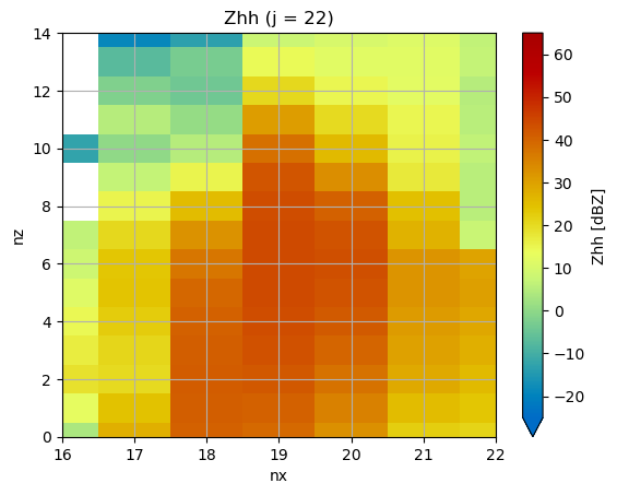
# 水平偏波反射強度 ZH (dBZ) の鉛直断面 (j = 22)
fig, ax = plt.subplots()
ds.Zhh[:,22,:].plot(ax=ax, cmap=pyart.graph.cm_colorblind.HomeyerRainbow, vmin=-25, vmax=65)
ax.set_xlim(16,22)
ax.set_ylim(0,14)
ax.set_title('$Z_{H}$ (j = 22)')
ax.grid()

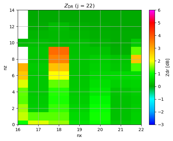
# 反射因子差 ZDR (dB) の鉛直断面 (j = 22)
fig, ax = plt.subplots()
ds.Zdr[:,22,:].plot(ax=ax, cmap=pyart.graph.cm.RefDiff, vmin=-3, vmax=6)
ax.set_xlim(16,22)
ax.set_ylim(0,14)
ax.set_title('$Z_\mathrm{DR}$ (j = 22)')
ax.grid()

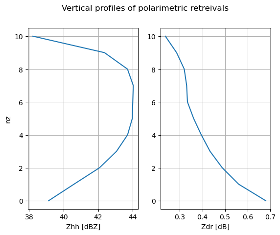
fig, axs = plt.subplots(ncols=2)
ds.Zhh[:11,22,19].plot(y='nz', ax=axs[0])
axs[0].grid()
ds.Zdr[:11,22,19].plot(y='nz', ax=axs[1])
axs[1].set_ylabel('')
axs[1].grid()
fig.suptitle('Vertical profiles of polarimetric retreivals')

まず、Spectral Bin Microphysics Model で確認した雨水混合比と同じ領域で、計算した水平偏波反射強度の水平分布を確認した。反射強度で見てもだいたい同じ位置で値のピークがある。

次に、y = 22 に沿った断面を示す。ここでは、水平偏波反射強度と反射因子差を示す。z = 10 がだいたい高度 5 km に相当する。Zhh > 30 dBZ の領域が x = 19 付近で 5 km を超えて分布している。同じ断面を反射因子差で見ると、反射強度の高い領域とは少しずれた部分に ZDR > 3 dB となる分布が計算されている。

Spectral Bin Microphysics Model の粒径分布の高度変化を確認した grid で水平偏波反射強度と反射因子差の鉛直分布を確認する。z < 4 では、反射強度は地上に向かって減少、反射因子差は地上に向かって微増していることがわかる。ここで、粒径分布とレーダー変数で示した Zhh と ZDR の式の形をよく見ると、Zhh は粒径の 6 乗、ZDR は粒子のアスペクト比にそれぞれ比例する。2 mm 未満の粒径の頻度が地上に向かって減少していたことは、Zhh が地上に向かって減少していることと整合的である。加えて、2 mm 以上の粒径の頻度が地上に向かってやや増加していたことは、ZDR が地上に向かって微増していることに対応していると考えることができる。これを言い換えると、雨粒は大きくなるほど扁平になるので、アスペクト比が大きくなるということを意味する。

以上のように、粒形分布に加えて二重偏波レーダー変数が算出できると、それぞれの特徴を相互に比較することが可能となる。加えて、観測データと直接比較も容易になる。

おわりに

今回は、CR-SIM を用いたレーダー変数の計算、それらの描画について試行した。有益なツールの開発・管理を行っている開発者の方々に謝意を示す。

参考文献

Oue, M., A. Tatarevic, P. Kollias, D. Wang, K. Yu, and A. M. Vogelmann, 2020: The Cloud-resolving model Radar SIMulator (CR-SIM) Version 3.3: description and applications of a virtual observatory, Geosci. Model Dev., 13, 1975–1998.

更新履歴

2024-01-20: 初稿

Miscellaneous — Jan 20, 2024

View / Make Comments

Made with ❤ and at Japan.